

The effectiveness of a RAG system depends intrinsically on how we chunk our corpus, yet the common practice of copying default configurations without measuring anything is a fundamental mistake.
There is no universally winning chunking strategy. Performance varies significantly with the domain, the structure of the text and the embedding model we use. So optimizing this stage isn't a trivial piece of initial setup, but an ongoing audit process.
The biggest risk is "blind truncation," a silent phenomenon where chunks exceed the model's window and get cut off during vectorization, degrading search without raising a single error. Auditing this behavior and measuring answer relevance with real queries is essential.
This process is a necessary investment of time and analysis that makes sure your system isn't capping its own potential right from the indexing phase.
The problem? You've never measured your splitter
You've probably seen this line of code, or one very much like it. It's in the repository of almost every RAG that has been in production for a while:
splitter = RecursiveCharacterTextSplitter(chunk_size=1000, chunk_overlap=200)
That line determines how each document is split before indexing and sets the size of the segments. It's a crucial setting: a RAG system doesn't retrieve whole documents, it retrieves chunks, so the quality of its answers depends directly on how it makes those cuts.
Those thousand characters and two hundred of overlap are usually inherited from the tutorial you followed when you started the project (and you know it!). Surprising as it may sound, I'm not going to criticize using that default. A well-tuned recursive splitter is hard to beat, something backed even by sources that would stand to gain from claiming otherwise, as I'll show below with hard data.
The enemy of chunking is something else, and it's far more uncomfortable: having picked that configuration once and never measured it.
One of the decisions with the biggest impact on answer quality is usually made by default, by replicating external configurations without any prior evaluation. The most common symptom is reacting to retrieval failures by swapping the splitter for a more complex algorithm, without first quantifying its real impact.
My position is that chunking isn't an architecture decision you make on day one. It's a parameter you measure against your own documents.
That's why this article won't give you a recommended chunk_size. It will show you how to measure yours. The failure isn't one of strategy or method. It's a failure of measurement.
Oh, and if you think RAG is dead, check out another post where we discuss exactly that.
Fixed windows: a surprisingly robust strategy
Recursive splitting with a fixed window and overlap can look like a very basic, beginner-level strategy, but it works. In 2024, Chroma published an evaluation of chunking strategies across five text collections (Smith & Troynikov, 2024). Curiously, the most-quoted result from that report is exactly the one that was least convenient for them.
Recursive chunking at 200 tokens achieved 88.1% recall. Surprisingly, Chroma's own semantic chunker comes in at 87.3%.
Worth pausing on: the study was done by a company that sells vector databases, and its results tell us that the tried-and-true heuristic retrieves slightly more than the sophisticated chunker the company itself proposes.
The authors' conclusion is the full concession: simple heuristics work well in practice when they're properly tuned.
There's a second, less-cited but decisive point to keep in mind. Evaluating chunking rigorously goes far beyond changing a parameter and checking that the demo still answers. The traditional standard calls for building a dataset (ground truth) on your own corpus, which is costly and hard to scale, but it isn't the only way. Today there are alternatives validated in the literature: from automated synthesis of test cases (Ragas, ARES), to isolated analysis of the retriever using classic information retrieval metrics like Hit Rate, MRR or NDCG (BEIR benchmark), to auditing contextual relevance with the LLM-as-a-judge paradigm.
Also, and this is an opinion with no data behind it, chunking is perceived as plumbing that comes before the interesting work. It gets dispatched in the first week of the project so the team can move on to prompt engineering, re-ranking or agentic systems as soon as possible.
Four strategies, one document: which one wins and what each one breaks
Let's use a simple analysis as an example, a toy exercise to illustrate the concepts. We're not trying to do deep research here, but to show the practical steps for evaluating our chunking and how some often-ignored factors affect answer quality.
I applied four chunking strategies to a single document: an internal policy on "Days off, vacation and absences.pdf" from Paradigma Digital. It has 9 pages and 18,638 characters, with headings, FAQs and numbered lists. The classic document at any company.
The document is internal, so I'll only publish the numbers and the cuts, not the text. The model used for the test is paraphrase-multilingual-MiniLM-L12-v2 (with a maximum sequence length of 128 tokens).
When evaluating how to chunk a document, we run into four main approaches, each with a different balance of cost, predictability and contextual coherence. As Figure 1 shows, these strategies produce very different size ranges on the same document, which directly shapes retrieval effectiveness:
- Fixed window: the cheapest and most predictable option. Because it splits on a rigid count, it ignores sentence structure. Its robustness depends almost entirely on overlap to recover context between chunks.
- Recursive: implements a hierarchy of separators (paragraphs, sentences, characters). This is, apparently, a notable improvement over fixed windows, since it tries to respect the logic of the text, producing more consistent chunks and a "cleaner" split that starts at the beginning of paragraphs.
- Structural: takes advantage of syntax (titles, headings) to extract units that make complete sense. It's extremely effective when extraction is accurate, but highly dependent on parser quality. Any typo can turn a stray line into a false heading, breaking the coherence of the blocks.
- Semantic: the most sophisticated, grouping text by similarity of meaning. It produces the most topically coherent blocks, but it's also the costliest and hardest to control, since chunk size stops being an adjustable parameter and becomes a consequence of the content, creating everything from noise (minimal blocks of 2 characters, as seen in Figure 1) to excessively long chunks.
There is no absolute winner. Each method wins at something and breaks something else depending on the nature of the text. The choice shouldn't be a lottery based on the method's popularity, but a decision grounded in how each strategy handles the information units in your corpus.
Analysis results
The first thing we can observe and analyze is chunk length for each strategy. This gives us an idea of how uneven the resulting sizes are, which is the first indicator of how each strategy affects the granularity of the information.
Figure 1 shows the range of results for the reference document.
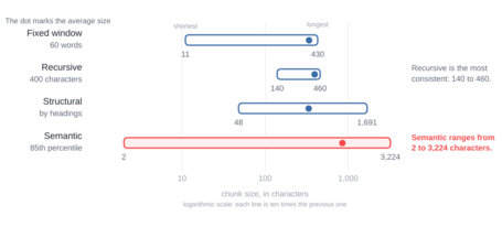
Figure 1 gives us more data on the process. Each strategy yields a specific number of chunks: 72, 56, 50 and 22, and none of the four deserves to be discarded outright. Fewer chunks is not a better indicator.
This brings us to the fundamental dilemma of granularity: a constant trade-off between overall context and fine detail. Chunks that are too small gain precision for direct queries, but risk losing the thread needed to understand the full answer.
Conversely, excessively long chunks preserve context but often "dilute" the relevant information, making it harder for the system to locate the specific fact. Finding the balance isn't an exact science but a fine-tuning exercise that depends entirely on how the information is structured in your corpus.
The table below also shows how many tokens each of those chunks takes up, compared with the 128-token window length set by the model used. This limit marks the threshold of the blind truncation phenomenon, which introduces a dangerous semantic bias:
This "blind truncation" phenomenon, illustrated in Figure 2, introduces a dangerous semantic bias by compromising the chunk's vector representation. It's a problem of "partial blindness": the LLM receives the full information, but the retrieval system, which acts as the input filter, never processed that information during the search phase. This sometimes explains why the system can retrieve an apparently relevant chunk based solely on its beginning, yet deliver a poor answer because the core of the information was in the discarded tokens.
| Strategy | No. of chunks | Avg. characters | Max | Tokens (max) |
|---|---|---|---|---|
| Fixed (60 words) | 72 | 336 | 430 | 100 |
| Recursive (400 char.) | 56 | 391 | 460 | 122 |
| Structural | 50 | 333 | 1,691 | 384 |
| Semantic | 22 | 845 | 3,224 | 761 |
Table 1. Comparison of the four chunking strategies applied to the document "Days off, vacation and absences.pdf".
And here's why this failure survives for years inside a production system: whatever exceeds the window is discarded at vectorization, with no error and no warning.
It's a completely silent process: no exceptions, warnings or errors in the system logs. The chunk enters the index, takes up its vector and behaves perfectly normally. Except that vector represents its first 128 tokens and nothing more.
The full text does reach the LLM, because it travels in the payload. But it took no part in the search. What decided whether that chunk got retrieved or not was a fragment of the fragment, which is an enormous loss of information.
Figure 2 illustrates this phenomenon. The 128-token threshold doesn't distinguish between effective and ineffective strategies. Instead, it cuts across the distribution of those that, by their nature, fit the document's structure better.
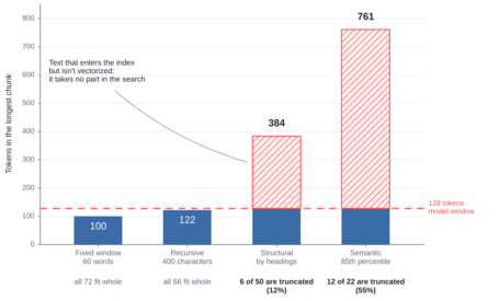
So before analyzing retrieval metrics or tuning window size, auditing truncation is a mandatory step. If your chunks are being blindly cut off by the embedding model, any later optimization will be in vain, because the system will be indexing incomplete information.
Evaluating this phenomenon is, ultimately, the first stress test to check whether your chunking strategy actually works or whether it's been limiting your RAG's potential from day one. That's the first piece of data worth having on the table before debating which strategy is best.
Calibrating chunk size: why the similarity score is not enough as a relevance criterion
In this case, only the fixed and recursive strategies let you set the chunk size. This calibration only makes sense with these strategies, which tend to be the most common when you start building a RAG system.
The same document was indexed with three size and overlap configurations, measured in words, and I ran a query of the kind any employee would ask: how many unused vacation days can be carried over, and until when?
The score in Table 2 is the cosine similarity between the question vector and the top-1 chunk vector, computed over an index built from scratch for each configuration. It doesn't measure whether the answer is complete, only the geometric closeness between the two.
| Size / overlap (words) | Chunks generated | Top-1 score | Contains the answer? |
|---|---|---|---|
| 30 / 5 | 124 | 0.6868 | No: returns 8-week leave entitlements |
| 60 / 15 | 72 | 0.7704 | Yes, but cut off at "before March 31 of the year" |
| 120 / 30 | 39 | 0.7690 | Yes, and complete: "of the current year" |
Table 2. Result of the pilot query on three size and overlap configurations, same document.
The results show three things at once:
- With chunks that are too small (30 words), the answer gets scattered across several pieces and the system returns text from a different page, a failure nothing fixes afterward.
- The score doesn't pick the right winner either: 60 words gets 0.7704 versus 0.7690 for 120 words, a difference within noise, and the one that "wins" is the one that cuts the answer in half, while the one that "loses" brings back the full deadline.
- Size determines cost: going from 30 to 120 words, chunks drop from 124 to 39, so there's less to index and compare, in exchange for sending more tokens with each query.
What this example teaches can be summed up in one sentence: a system can return a high score, on the right document and the right page, and still deliver an answer that's missing information.
That missing information may get "filled in" by the LLM in its response, which is yet another source of hallucinations we need to watch for.
Now the fine print, before anyone writes it in the comments. This is one query, one document and one top-1. In other words, it illustrates a mechanism; it doesn't measure it. With a different question, the order of the scores can change, and this table's winner is not a size recommendation for anyone. It's proof that you need to measure your corpus rather than copy anyone else's configuration.
What the latest large-scale research says
So far we've looked at a "toy" case: one document, one quick experiment and one sample query. Time to test these observations against evidence at scale and see whether emerging techniques really overcome the truncation problems we've detected.
In this study by Shaukat et al. (2026), researchers measured 1,080 configurations, applying 36 chunking strategies across six domains and five embedding models, with retrieval isolated from the rest of the system. After all that volume, the study's results confirm what we've been saying in this post: there is no single winner. For example, dynamic chunking dominates in Biology, Health and Physics. Paragraph grouping wins in Legal and Mathematics. And in Agriculture, no method stands out clearly.
One fundamental conclusion comes out of this research: there is no universal strategy, because the effectiveness of each method depends intrinsically on the domain and the corpus.
It's also a mistake to try to compensate for a poor chunking strategy by using more advanced embedding models.
Since chunking and embeddings work multiplicatively rather than as mutually exclusive alternatives, bad chunking will irreparably limit the performance of any model, regardless of its cost or sophistication.
The question that does have an answer
The question almost all of us arrive with is: what's the best chunking strategy? It's the wrong question, and as we've seen in this post, it still has no answer.
The ideal strategy isn't fixed: its performance shifts with the domain, the embedding model and the structure of your documents.
That's why the key question isn't which one is best, but how much accuracy we're losing by not auditing our own chunking configuration.
Answering it takes time and deliberate analysis. Spending a few days auditing how many chunks exceed the model's window, preparing representative queries with business experts and testing different configurations, among other things, is an investment worth making. You don't need a complex benchmark. What you need is commitment.
The essence of this article boils down to one maxim: don't adopt a chunking strategy out of inertia, measure yours.
And if you know someone who built their RAG a year and a half ago and hasn't opened the file where the splitter lives since, share this with them. They have the most to gain from spending a few days on this review.
References
- Es, S., James, J., Anke, L. E., & Schockaert, S. (2024, March). Ragas: Automated evaluation of retrieval augmented generation. In Proceedings of the 18th conference of the european chapter of the association for computational linguistics: system demonstrations (pp. 150-158).
- Ford, D. (2024, September 19). Introducing contextual retrieval. Anthropic.
- Günther, M., Mohr, I., Williams, D. J., Wang, B., & Xiao, H. (2024). Late chunking: Contextual chunk embeddings using long-context embedding models. arXiv:2409.04701.
- Lu, W., Chen, K., Qiao, R., & Sun, X. (2025). HiChunk: Evaluating and enhancing retrieval-augmented generation with hierarchical chunking [Preprint]. arXiv:2509.11552.
- Merola, C., & Singh, J. (2025). Reconstructing context: Evaluating advanced chunking strategies for retrieval-augmented generation. Second Workshop on Knowledge-Enhanced Information Retrieval (KEIR), ECIR 2025. Preprint: arXiv:2504.19754.
- Saad-Falcon, J., Khattab, O., Potts, C., & Zaharia, M. (2024, June). Ares: An automated evaluation framework for retrieval-augmented generation systems. In Proceedings of the 2024 Conference of the North American Chapter of the Association for Computational Linguistics: Human Language Technologies (Volume 1: Long Papers) (pp. 338-354).
- Shaukat, M. A., Adnan, M., & Kuhn, C. C. N. (2026). A systematic investigation of document chunking strategies and embedding sensitivity [Preprint]. arXiv:2603.06976.
- Smith, B., & Troynikov, A. (2024). Evaluating chunking strategies for retrieval [Technical report]. Chroma.
- Thakur, N., Reimers, N., Rücklé, A., Srivastava, A., & Gurevych, I. (2021). Beir: A heterogenous benchmark for zero-shot evaluation of information retrieval models. arXiv preprint arXiv:2104.08663.
- Zheng, L., Chiang, W. L., Sheng, Y., Zhuang, S., Wu, Z., Zhuang, Y., ... & Stoica, I. (2023). Judging llm-as-a-judge with mt-bench and chatbot arena. Advances in neural information processing systems, 36, 46595-46623.

Jorge C. Barrios
Artificial intelligence has been at the center of my day-to-day for ten years, and I still approach it with a fascination for its science and fundamentals. I’m naturally curious and passionate about continuous learning. I still happily lose myself in books and theory, turning concepts, data and research into useful technology.
View more of Jorge C..More thoughts about this.
Read more.
When AI Designs What You Don't Need.

Retrieval Augmented Generation and its corporate usage.

How will machines understand us in the future?

Unfiltered Artificial Intelligence: 3 Resources to Harness Its Full Potential.

Comments are moderated and will only be visible if they add to the discussion in a constructive way. If you disagree with a point, please, be polite.

Tell us what you think.