Deep Learning with neural networks is currently one
of the most promising branches of artificial intelligence. This innovative
technology is commonly used in applications such as image recognition, voice
recognition and machine translation, among others.

There are several options out there in terms of technologies and libraries, Tensorflow – developed by Google – being the most widespread nowadays.

However, today we are going to focus on PyTorch, an emerging alternative that is quickly gaining traction thanks to its ease of use and other advantages, such as its native ability to run on GPUs, which allows traditionally slow processes such as model training to be accelerated. It is Facebook’s main library for deep learning applications.

Its basic elements are tensors, which can be equated to vectors with one or several dimensions.

Artificial Neural Networks (ANNs)

An Artificial Neural Network is a system of nodes that are interconnected in an orderly manner and arranged in layers and through which an input signal travels to produce an output. They receive this name because they aim to simply emulate the workings of the biological neural networks in animal brains.

They are made up of an input layer, one or more hidden layers and an output
layer, and can be trained to ‘learn’ how to recognize certain patterns. This
characteristic is what makes them be considered a part of ecosystem of
technologies known as artificial
intelligence.

ANNs are several decades old, but have attained great importance in recent years due to the increased availability of the large amounts of data and computing power that are required for them to be used to solve complex problems.

They have entailed a historical milestone in applications that have been traditionally refractory to classical, rule-based programming, such as image or voice recognition.

Installing PyTorch

If we have the Anaconda environment installed, PyTorch is installed with the following command:

console

conda install pytorch torchvision -c pytorch

Otherwise, we
can use pip as follows:

console

pip3 install torch torchvision

Example of an ANN

Let us look at a simple case of image sorting by deep learning using the well-known MNIST dataset, which contains images of handwritten numbers from 0 to 9.

Loading the dataset

import torch, torchvision

In order to be able to use the dataset with PyTorch, it must be transformed into a tensor. To do this, we must define a T transformation that will be used in the loading process. We must also define a DataLoader, a Python generator object whose purpose is to provide images in batch_size groups of images at the same time.

Note: It is typical in neural network training to update the parameters every N inputs instead of every individual input. However, excessively increasing the group size could end up taking up too much RAM in the system.

T = torchvision.transforms.Compose([torchvision.transforms.ToTensor()])
images = torchvision.datasets.MNIST('mnist_data', transform=T,download=True)
image_loader = torch.utils.data.DataLoader(images,batch_size=128)

Defining the topology of the ANN

Next, we need to decide what topology our network is going to have. An ANN consists
of an input layer, one or more intermediate or, as they are commonly known,
hidden layers, and an output layer.

The number of hidden layers, as well as the amount of neurons in them,
depends on the complexity and the type of the problem. In this simple case, we are going
to implement two hidden layers of 100 and 50 neurons respectively.

The class we must create is inherited from the nn.Module class. Additionally, we will need to initialize the methods of the superclass.

import torch.nn as nn
#definimos la red neuronal
class Classifier(nn.Module):
def __init__(self):
super(Classifier,self).__init__()
self.input_layer = nn.Linear(28*28,100)
self.hidden_layer = nn.Linear(100,50)
self.output_layer = nn.Linear(50,10)
self.activation = nn.ReLU()
def forward(self, input_image):
input_image = input_image.view(-1,28*28)                     #convertimos la imagen a vector
output = self.activation(self.input_layer(input_image)) #pasada por la capa entrada
output = self.activation(self.hidden_layer(output))   #pasada por la capa oculta
output = self.output_layer(output)                    #pasada por la capa de salida
return output

The input layer

It has as many neurons as there is data in our samples. In this case, the inputs are images of 28x28 pixels showing the handwritten numbers. Therefore, our input layer will comprise 28x28 neurons.

The output layer

It has as many possible outputs as there are classes in our data – 10 in this case (digits from 0 to 9). For every input, the output nodes will yield a value – the greater of which is identified with the detected output class.

The activation function

This function defines the output of a node according to an input or a set of inputs. In this case, we will use the simple ReLU (Rectified Linear Unit) function:

% block:caption
% image:https://www.paradigmadigital.com/wp-content/uploads/2019/03/Pytorch-1.png
% caption:y=max(0,x)

% endblock

The ‘Forward’ propagation function

This function defines how the calculations will be performed from the input data, which will go through the different layers, to the output. It starts by flattening the input from a two-dimensional 28x28-pixel tensor to a one-dimensional tensor of 784 values that are transferred to the input layer using the view function.

These values will be then propagated to the hidden layers by means of the activation function and, finally, to the output layer, which will return the result.

Training the ANN

In order to successfully train our network, we need to define some parameters.

from torch import optim
import numpy as np
classifier = Classifier() #instanciamos la RN
loss_function = nn.CrossEntropyLoss() #función de pérdidas
parameters = classifier.parameters()
optimizer = optim.Adam(params=parameters, lr=0.001) #algoritmo usado para optimizar los parámetros
epochs = 3 #número de veces que pasamos cada muestra a la RN durante el entrenamiento
iterations = 0 #número total de iterations para mostrar el error
losses = np.array([]) #array que guarda la pérdida en cada iteración

First we will instantiate an object of the previously defined class, which is termed a classifier. Apart from that, we will need:

A loss function

We will use this function to optimize the parameters; their value will be minimized during the network training phase. There are many loss functions available for PyTorch. In this case, we will use cross entropy loss, which is recommended for multiclass classification situations such as the one we are discussing in this post.

An optimizer

This object receives the model and learning rate parameters and iteratively updates them according to the gradient of the loss function during the training of the network. In this case, we have used an Adam algorithm, although others can be used as well.

Epoch sets the number of times the dataset will be passed through the ANN for training purposes. This practice is a typical convention in the training of deep learning systems. The other parameters will be used to store and subsequently display the results.

Training loop

from torch.autograd import Variable #necesario para calcular gradientes
for e in range(epochs):
for i, (images, tags) in enumerate(image_loader):
images, tags = Variable(images), Variable(tags) #Convertir a variable para derivación
output = classifier(images) #calcular la salida para una imagen
classifier.zero_grad() #poner los gradientes a cero en cada iteración
error = loss_function(output, tags) #calcular el error
error.backward() #obtener los gradientes y propagar
optimizer.step() #actualizar los pesos con los gradientes
iterations += 1
losses = np.append(losses,error.item())

Training will takes place the number of times that is set in the epochs
variable, which is reflected in the outer loop. The following steps will be then
carried out:

1. Extracting the images and their tags from the previously defined image_loader object.
2. Transforming the images and tags to the Variable type, since this data type that allows us to store the gradients in order to thus be able optimize the parameters or weights of the model.
3. Transferring the input (images) to the classifier model.
4. Resetting the gradients. If we do not perform this operation, the gradients would start accumulating, giving rise to erroneous classifications.
5. Calculating the loss, which is a measure of the difference between the forecast and the tags that are present.
6. With the backward() function, obtaining and propagating the gradients.
7. Updating the weights with the optimizer object. This is known as the backpropagation method.
8. Saving the number of iterations and the losses in each one of them in order to be able to display them.

Results

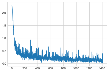
Now we are ready to see the outcome of our training! To this end, we will use the matplotlib library. Since we saved the iterations and the loss, we just have to plot them in a graph to have an idea of how much progress our ANN has made.

import matplotlib.pyplot as plt
plt.style.use('seaborn-whitegrid')
#vemos las pérdidas en cada iteración de forma gráfica
plt.plot(np.arange(iterations),losses)

It can be seen in the graph above how the classification error has decreased as the ANN has been trained.

Conclusion

There are
several – both free and proprietary – options out there for programming ANNs. Although
Google’s TensorFlow is still the undisputed market leader, little by little
interesting alternatives are emerging that might add value to the ecosystem due
to having native compatibilities, their ease of use, and so on.